Asymptotics

lec13 Asymptotics I

我们可以从两个不同的角度来考虑编写高效程序的过程：

1. 编程成本（截至目前课程中的所有费用）
   1. 您开发程序需要多长时间？
   2. 阅读或修改代码有多容易？
   3. 您的代码的可维护性如何？ （非常重要——大部分成本来自维护和可扩展性，而不是开发！）
2. 执行成本（从此时开始课程中的所有内容）
   1. 时间复杂度：你的程序执行需要多少时间？
   2. 空间复杂度：您的程序需要多少内存？

Asymptotic（渐近） Analysis In most cases, we care only about asymptotic behavior, i.e. what happens  for very large N.

Algorithms which scale well (e.g. look like lines) have better asymptotic runtime behavior than algorithms that scale relatively poorly (e.g. look like parabolas).

Computing Worst Case Order of Growth：

1. Only consider the worst case.
2. Pick a representative operation (a.k.a. the cost model).
3. Ignore lower order terms.
4. Ignore multiplicative constants.

the tightest Ω and big O bounds.

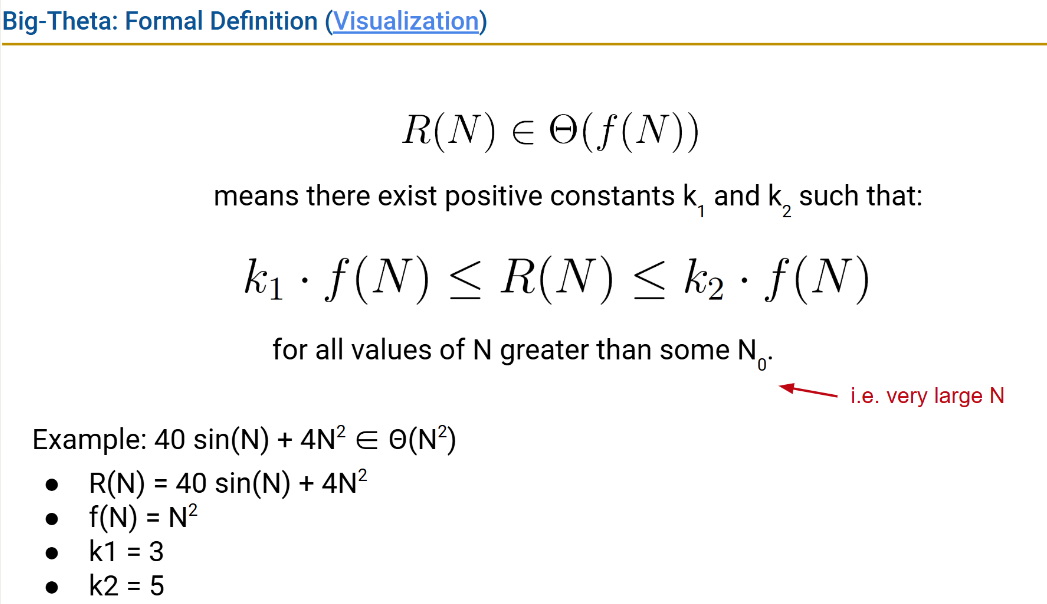
Big Theta (a.k.a. Order of Growth):

Formal Definition : For some function 𝑅(𝑁) with order of growth 𝑓(𝑁), we write that: 𝑅(𝑁)∈Θ(𝑓(𝑁)) and there exists some positive constants $𝑘_1​, 𝑘_2$ such that… $𝑘_1⋅𝑓(𝑁)≤𝑅(𝑁)≤𝑘_2⋅𝑓(𝑁)$ for all values 𝑁 greater than some $𝑁_0$ (a very large 𝑁).

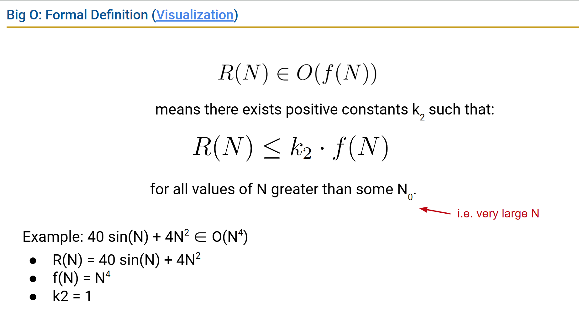
Big O

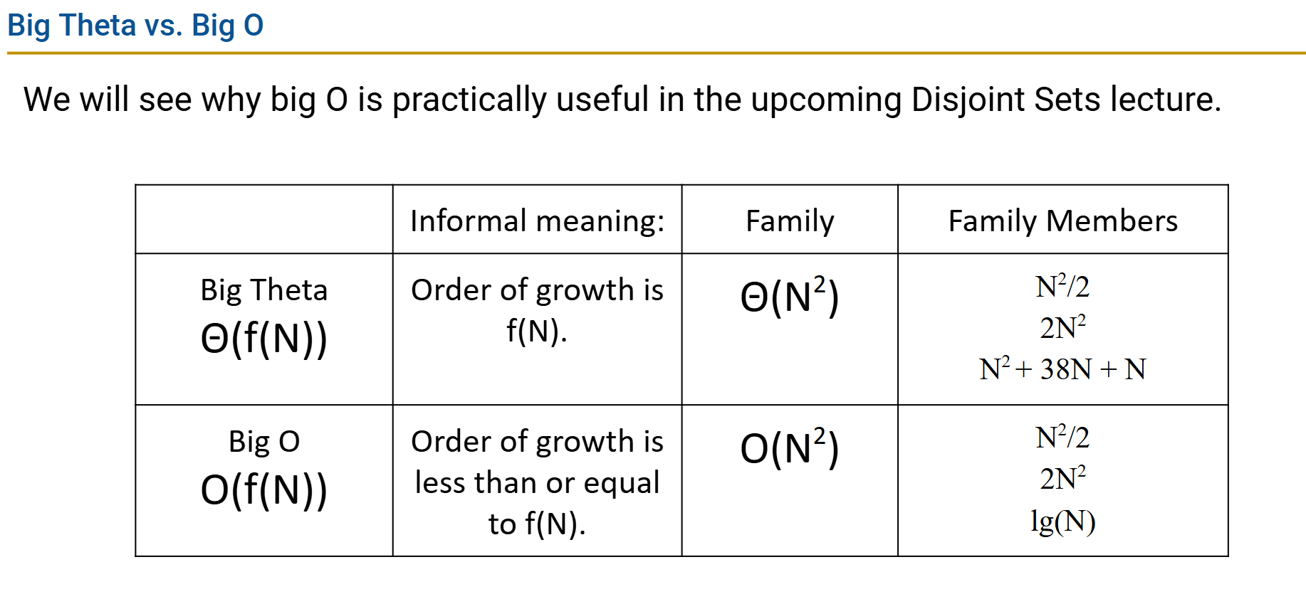
Whereas Big Theta can informally be thought of as something like “equals”, Big O can be thought of as “less than or equal”.

Example, the following are all true:

• N3 + 3N4 ∈ O(N6)
• N3 + 3N4 ∈ O(N!)

R(N)∈O(f(N)) means that there exists positive constant $𝑘_2$ ​ such that: $𝑅(𝑁)≤𝑘_2⋅𝑓(𝑁)$ for all values of 𝑁 greater than some $𝑁_0$ (a very large 𝑁).

To summarize this chapter:

• Given a piece of code, we can express its runtime as a function 𝑅(𝑁)
  • 𝑁 is a property of the input of the function often representing the size of the input
• Rather than finding the exact value of 𝑅(𝑁), we only worry about finding the order of growth of 𝑅(𝑁).

Remember that asymptotics only apply to very large inputs!

lec15 Asymptotics II

Techniques: No Magic Shortcuts

But there are a few useful techniques and things to know:

• Find exact sum
• Write out examples 
• Draw pictures

Method 1: Finding the Bound Visually

Method 2: Finding the Bound Mathematically 𝐶(𝑁)=1+2+4+…+𝑁=2𝑁−1， so the runtime is 𝜃(𝑁).

two important sums you’ll see very often:

• Sum of First Natural Numbers: 1+2+3+…+𝑄=𝑄(𝑄+1)/2=Θ(𝑄​2​​)
• Sum of First Powers of 2: 1+2+4+8+…+𝑄=2𝑄−1=Θ(𝑄)

$1 + 2 + 3 + 4 + 5 + … + N = Θ(N^2)$ $1 + 2 + 4 + 8 + 16 + … + N = Θ(N)$

General case: $1 + 2 + 3 + 4 + 5 + … + f(N) = Θ(f(N)^2)$ $1 + 2 + 4 + 8 + 16 + … + f(N) = Θ(f(N))$ (any geometric factor between terms, ie. 1 + 3 + 9 + …)

$log_2 n = \frac{log n}{log 2}$

A couple properties worth knowing (see below for proofs):

• $⌊𝑓(𝑁)⌋=Θ(𝑓(𝑁))$
• $⌈𝑓(𝑁)⌉=Θ(𝑓(𝑁))$
• $𝑙𝑜𝑔_𝑝(𝑁)=Θ(𝑙𝑜𝑔_𝑞(𝑁))$

Takeaways 

• There are no magic shortcuts for analyzing code runtime.
• 𝑁2 vs. 𝑁𝑙𝑜𝑔(𝑁) is an enormous difference.
• Going from 𝑁𝑙𝑜𝑔(𝑁)) to 𝑁 is nice, but not a radical change.

Binary search the order of growth of the worst case runtime: $log_2N$ (the overall runtime then is order 𝑙𝑜𝑔2(𝑁).